A Journey Through Fastbook (AJTFB) - Chapter 9: Tabular Modeling

fastai

fastbook

tabular

structured

decision trees

random forest

embeddings

categorical variables

boosting

gdbt

xgboost

In chapter of 8 of “Deep Learning for Coders with fastai & PyTorch” we learned that the neural network version of of collaborative model is in fact built on something called TabularModel, and that in fact, an EmbeddingNN is nothing but a TabularModel without any continuous (or real) numbers. “Structured” or “tabular” data describes datasets that look like an Excel spreadsheet or a relational database table, of which, it may be a composed of both categorical and/or real numbers. Working with such data is the subject of chapter 9, so lets go!

Author

Wayde Gilliam

Published

April 25, 2022

Other posts in this series:
A Journey Through Fastbook (AJTFB) - Chapter 1
A Journey Through Fastbook (AJTFB) - Chapter 2
A Journey Through Fastbook (AJTFB) - Chapter 3
A Journey Through Fastbook (AJTFB) - Chapter 4
A Journey Through Fastbook (AJTFB) - Chapter 5
A Journey Through Fastbook (AJTFB) - Chapter 6a
A Journey Through Fastbook (AJTFB) - Chapter 6b
A Journey Through Fastbook (AJTFB) - Chapter 7
A Journey Through Fastbook (AJTFB) - Chapter 8

Tabular Modeling

What is it?

“Tabular modeling takes data in the form of a table (like a spreadsheet or CSV). The objective is to predict the value of one column based on the values in the other columns.” Tabular data is also called “structured data” while “unstructured data” represents things like text, images, audio, etc…

Why is it important?

Though it is reported that 80-90% of data is unstructured (think images, text, audio), ironically, it appears that the vast majority of “real world” machine learning is concerened with tabular/structured data.

If you are just starting out with Data Science you should know that still the vast majority of DS problems in the industry concern structured/tabular data. This is what you should focus on in order to make a professional inroad.

1/3
— Bojan Tunguz (@tunguz) February 23, 2022

Note

And here’s the good news … “recent studies have shown that the vast majority of datasets can be be modeled with just two methods.”

What are they?

For structured data, ensembles of decision trees (e.g., random forests and gradient boosting machines like XGBoost).
For unstructured data, multilayered neural networks learned with SGD.

Note

“… ensembles of decision trees tend to train faster, are often easier to interpret, do not require special GPU hardware for inference at scale, and often require less hyperparameter tuning.

Important

Since a “critical step of interpreting a model of tabular data is significantly easier for decesion tree ensembles … ensembles of decision trees are our first approach for analyzing a new tabular dataset”

Important

Neural networks will considered when “there are some high-cardinality categorical variables” or there are columns with unstructured data. A example of a high “cardinality” (e.g., the number of discrete levels representing the categories) would be something like zip code.

See pages 282-284 for more discussion on the pros/cons of decision trees and neural networks for tabular data.

Categorical Embeddings

Continuous v. Categorical

Continuous variables “contain a real numbers that be fed into a model directly and are meaningful in and out of themselves. Examples include”age” and “price”.

Categorical variables “contain a number of discrete levels, such as ‘movie ID,’ for which addition and multiplication don’t have any meaning (even if they’re stored as numbers). Other examples include dates, columns indicating”sex”, “gender”, “department”, etc…

How do we represent “categorical” data?

We learned this in chapter 8, we represent such data via entity embeddings.

Important

Entity embeddings allow for a more complex and learnt numerical representation of a thing. This representation is likely task/data specific to one degree or another such that “Sunday” may have one representation in a task predicting how many hours people work on a day, and another for a task attempting to predict the number of trades that will be executed on each day of the week.

Note

“… by mapping similar values close to each other in the embedding space it reveals the intrinsic properties of the categorical variable. [It] is especially useful for datasets with lots of high cardinality features.. See pp.278-282 for examples of this in relation to the Rossmann sales competition on kaggle.

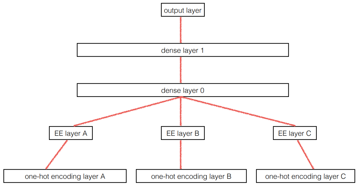
Because “an embedding layer is exactly equivalent to placing an ordinary linear layer after every one-hot-encoded input layer … the embedding transforms the categorical variables into inputs that are both continuous and meaningful.”

In other words …

Important

“… we provide the model fundamentally categorical data about discrete entities … and the model learns an embedding for these entities that defines a continuous notion of distance between them.”

Note

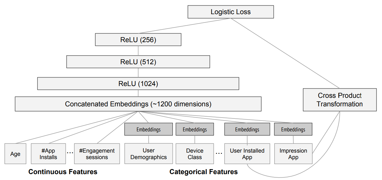
Given all this, “we can combine our continous embedding values with truly continuous input data [by just concatentating] the variables and feed[ing] the concatenation into our final dense layers. For an example of this, see the “Wide & Deep Learning for Recommender Systems” paper. See the below from page 282 on what that approach looks like.

Imports

from kaggle import api
from dtreeviz.trees import *
from fastai.tabular.all import *
from IPython.display import Image, display_svg, SVG
from pandas.api.types import is_string_dtype, is_numeric_dtype, is_categorical_dtype
from sklearn.ensemble import RandomForestRegressor
from sklearn.tree import DecisionTreeRegressor, export_graphviz

pd.options.display.max_rows = 20
pd.options.display.max_columns = 8

Data preparation

Step 1: Get the data

We’ll be getting the data from kaggle. If you’re running on colab, check out these instructions for getting setup with the kaggle API

path = Path("bluebook")
path

Path('bluebook')

if not path.exists():
    path.mkdir()
    api.competition_download_cli("bluebook-for-bulldozers", path=path)
    file_extract(path / "bluebook-for-bulldozers.zip")

path.ls(file_type="text")

Downloading bluebook-for-bulldozers.zip to bluebook

100%|██████████| 48.4M/48.4M [00:00<00:00, 112MB/s]

(#7) [Path('bluebook/Machine_Appendix.csv'),Path('bluebook/Test.csv'),Path('bluebook/ValidSolution.csv'),Path('bluebook/median_benchmark.csv'),Path('bluebook/TrainAndValid.csv'),Path('bluebook/Valid.csv'),Path('bluebook/random_forest_benchmark_test.csv')]

Step 2: EDA

Important

“In any sort of data science work, it’s important to look at your data directly to make sure you understand the format, how it’s stored, what types of values it holds, etc.”

Tip

“… it’s a good idea to also specify low_memory=False unless Pandas acutally runs out of memory.” The default = True (will look only at the first few rows of data to infer column datatypes).

train_df = pd.read_csv(path / "TrainAndValid.csv", low_memory=False)
test_df = pd.read_csv(path / "Test.csv", low_memory=False)

train_df.columns

Index(['SalesID', 'SalePrice', 'MachineID', 'ModelID', 'datasource',
       'auctioneerID', 'YearMade', 'MachineHoursCurrentMeter', 'UsageBand',
       'saledate', 'fiModelDesc', 'fiBaseModel', 'fiSecondaryDesc',
       'fiModelSeries', 'fiModelDescriptor', 'ProductSize',
       'fiProductClassDesc', 'state', 'ProductGroup', 'ProductGroupDesc',
       'Drive_System', 'Enclosure', 'Forks', 'Pad_Type', 'Ride_Control',
       'Stick', 'Transmission', 'Turbocharged', 'Blade_Extension',
       'Blade_Width', 'Enclosure_Type', 'Engine_Horsepower', 'Hydraulics',
       'Pushblock', 'Ripper', 'Scarifier', 'Tip_Control', 'Tire_Size',
       'Coupler', 'Coupler_System', 'Grouser_Tracks', 'Hydraulics_Flow',
       'Track_Type', 'Undercarriage_Pad_Width', 'Stick_Length', 'Thumb',
       'Pattern_Changer', 'Grouser_Type', 'Backhoe_Mounting', 'Blade_Type',
       'Travel_Controls', 'Differential_Type', 'Steering_Controls'],
      dtype='object')

describe() is a method that gives you some basic stats for each column.

train_df.describe().T

	count	mean	std	min	25%	50%	75%	max
SalesID	412698.0	2.011161e+06	1.080068e+06	1139246.0	1421897.75	1645852.5	2261012.50	6333349.0
SalePrice	412698.0	3.121518e+04	2.314174e+04	4750.0	14500.00	24000.0	40000.00	142000.0
MachineID	412698.0	1.230061e+06	4.539533e+05	0.0	1088593.25	1284397.0	1478079.25	2486330.0
ModelID	412698.0	6.947202e+03	6.280825e+03	28.0	3261.00	4605.0	8899.00	37198.0
datasource	412698.0	1.351694e+02	9.646749e+00	121.0	132.00	132.0	136.00	173.0
auctioneerID	392562.0	6.585268e+00	1.715841e+01	0.0	1.00	2.0	4.00	99.0
YearMade	412698.0	1.899050e+03	2.921902e+02	1000.0	1985.00	1995.0	2001.00	2014.0
MachineHoursCurrentMeter	147504.0	3.522988e+03	2.716993e+04	0.0	0.00	0.0	3209.00	2483300.0

advanced_describe() is a method I created that builds on top of the default describe() method to include stats on missing and unique values (which are both very helpful in terms of cleanup, understanding potential issues, and in determining the size of your embeddings for categorical data). For categorical variables with few discrete levels, this method will also show you what they are.

advanced_describe(train_df)

	count	mean	std	min	...	unique	unique%	unique_values	dtype
SalesID	412698	2011161.16364	1080067.724498	1139246.0	...	412698	7786.75	NaN	int64
SalePrice	412698	31215.181414	23141.743695	4750.0	...	954	18.00	NaN	float64
MachineID	412698	1230061.436646	453953.25795	0.0	...	348808	6581.28	NaN	int64
ModelID	412698	6947.201828	6280.824982	28.0	...	5281	99.64	NaN	int64
datasource	412698	135.169361	9.646749	121.0	...	6	0.11	[121, 132, 136, 149, 172, 173]	int64
...	...	...	...	...	...	...	...	...	...
Backhoe_Mounting	80712	NaN	NaN	NaN	...	3	0.06	[nan, None or Unspecified, Yes]	object
Blade_Type	81875	NaN	NaN	NaN	...	11	0.21	[nan, PAT, None or Unspecified, Semi U, VPAT, Straight, Angle, No, U, Landfill, Coal]	object
Travel_Controls	81877	NaN	NaN	NaN	...	8	0.15	[nan, None or Unspecified, Differential Steer, Lever, Finger Tip, 2 Pedal, Pedal, 1 Speed]	object
Differential_Type	71564	NaN	NaN	NaN	...	5	0.09	[Standard, nan, Limited Slip, No Spin, Locking]	object
Steering_Controls	71522	NaN	NaN	NaN	...	6	0.11	[Conventional, nan, Command Control, Four Wheel Standard, Wheel, No]	object

53 rows × 14 columns

Step 3: Preprocessing

Handling Ordinal columns

Tip

“… a good next step is to handle ordinal columns … columns containing strings or similar, **but where those strings have a natural ordering.”

train_df.ProductSize.unique()

array([nan, 'Medium', 'Small', 'Large / Medium', 'Mini', 'Large',
       'Compact'], dtype=object)

Important

“tell Pandas about a suitable ordering of these levels”

sizes = ["Large", "Large / Medium", "Medium", "Small", "Mini", "Compact"]
train_df.ProductSize = train_df.ProductSize.astype("category")
train_df.ProductSize = train_df.ProductSize.cat.set_categories(
    sizes, ordered=True
)  # note: "inplace=True" is depreciated as of 1.30
train_df.ProductSize.unique()

[NaN, 'Medium', 'Small', 'Large / Medium', 'Mini', 'Large', 'Compact']
Categories (6, object): ['Large' < 'Large / Medium' < 'Medium' < 'Small' < 'Mini' < 'Compact']

Handling Your Dependent Variable(s)

Tip

Update the dependent variable to suit your objective.

“You should think carefully about which metric, or set of metrics, actually measures the notion of model quality that matters to you … in this case, Kaggle tells us [our measure is] root mean squared log error (RMLSE)” and because of this we need to make our target the log of the price “so that the m_rmse of that value will give us what we ultimately need.”

dep_var = "SalePrice"
train_df[dep_var] = np.log(train_df[dep_var])

Handling Dates

Important

“… enrich our representation of dates”

Dates are “different from most ordinal values in that some dates are qualitatively different from others in a way that is often relevant to the systems we are modeling.” As such, we want the model to know if whether the day is a holiday, or part of the weekend, or in a certain month, etc… is important. To do this, “we **replace every date column with a set of date metadata columns, such as holiday, day of week, and month” = categorical data that might be very useful!

Can use fastai’s add_datepart() function to do this.

Important

Apply same preprocessing to both your train/evaluation and test sets!

train_df = add_datepart(train_df, "saledate")
test_df = add_datepart(test_df, "saledate")

[col for col in train_df.columns if col.startswith("sale")]

['saleYear',
 'saleMonth',
 'saleWeek',
 'saleDay',
 'saleDayofweek',
 'saleDayofyear',
 'saleIs_month_end',
 'saleIs_month_start',
 'saleIs_quarter_end',
 'saleIs_quarter_start',
 'saleIs_year_end',
 'saleIs_year_start',
 'saleElapsed']

Handling Strings and Missing Data

For this we can use fastai’s TabularPandas class (allows us to apply TabularProc transforms to the DataFrame it wraps to do things like fill missing values, make columns categorical, etc…).

Categorify: “a TabularProc that replaces a column with a numeric categorical column”

FillMissing: “a TabularProc that replaces missing values with the median of the column, and **creates a new Boolean column that is set to True for any row where the value was missing. You can change this fill strategy via thefill_strategy` argument.

procs = [Categorify, FillMissing]

Creating our `TabularPandas`

Step 1: Define our continuous and categorical columns

We need to tell TabularPandas what columns are continumous and which are categorical, and we can use fastai’s cont_cat_split to do that like so …

cont, cat = cont_cat_split(train_df, 1, dep_var=dep_var)

Step 2: Define our training and validation splits

What is the difference between validation and test sets again?

Recall that a validation set “is data we hold back from training in order to ensure that the training process does not overfit on the training data” … while a test set “is data that is held back from ourselves in order to ensure that we don’t overfit on the validation data as we export various model architectures and hyperparameters.”

Important

“define our validation data so that it has the same sort of relationship wot the training data as the test set will have.”

Because this is a time series problem, we’ll make the validation set include data for the last 6 months of the full training set, and the training set everything before that. See p.291 for more on this!

cond = (train_df.saleYear < 2011) | (train_df.saleMonth < 10)
train_idxs = np.where(cond)[0]
valid_idxs = np.where(~cond)[0]

splits = (list(train_idxs), list(valid_idxs))

Step 3: Build our `TabularPandas` object

And finally, we instantiate our TabularPandas object, passing in our data, procs, splits and dependent variables as such.

to = TabularPandas(train_df, procs, cat, cont, y_names=dep_var, splits=splits)
type(to)

fastai.tabular.core.TabularPandas

Note

“A TabularPandas behaves a lot like a fastai Datasets object, including train and valid attributes”

len(to.train), len(to.valid)

(404710, 7988)

to.show(3)

	UsageBand	fiModelDesc	fiBaseModel	fiSecondaryDesc	fiModelSeries	fiModelDescriptor	ProductSize	fiProductClassDesc	state	ProductGroup	ProductGroupDesc	Drive_System	Enclosure	Forks	Pad_Type	Ride_Control	Stick	Transmission	Turbocharged	Blade_Extension	Blade_Width	Enclosure_Type	Engine_Horsepower	Hydraulics	Pushblock	Ripper	Scarifier	Tip_Control	Tire_Size	Coupler	Coupler_System	Grouser_Tracks	Hydraulics_Flow	Track_Type	Undercarriage_Pad_Width	Stick_Length	Thumb	Pattern_Changer	Grouser_Type	Backhoe_Mounting	Blade_Type	Travel_Controls	Differential_Type	Steering_Controls	saleIs_month_end	saleIs_month_start	saleIs_quarter_end	saleIs_quarter_start	saleIs_year_end	saleIs_year_start	auctioneerID_na	MachineHoursCurrentMeter_na	SalesID	MachineID	ModelID	datasource	auctioneerID	YearMade	MachineHoursCurrentMeter	saleYear	saleMonth	saleWeek	saleDay	saleDayofweek	saleDayofyear	saleElapsed	SalePrice
0	Low	521D	521	D	#na#	#na#	#na#	Wheel Loader - 110.0 to 120.0 Horsepower	Alabama	WL	Wheel Loader	#na#	EROPS w AC	None or Unspecified	#na#	None or Unspecified	#na#	#na#	#na#	#na#	#na#	#na#	#na#	2 Valve	#na#	#na#	#na#	#na#	None or Unspecified	None or Unspecified	#na#	#na#	#na#	#na#	#na#	#na#	#na#	#na#	#na#	#na#	#na#	#na#	Standard	Conventional	False	False	False	False	False	False	False	False	1139246	999089	3157	121	3.0	2004	68.0	2006	11	46	16	3	320	1.163635e+09	11.097410
1	Low	950FII	950	F	II	#na#	Medium	Wheel Loader - 150.0 to 175.0 Horsepower	North Carolina	WL	Wheel Loader	#na#	EROPS w AC	None or Unspecified	#na#	None or Unspecified	#na#	#na#	#na#	#na#	#na#	#na#	#na#	2 Valve	#na#	#na#	#na#	#na#	23.5	None or Unspecified	#na#	#na#	#na#	#na#	#na#	#na#	#na#	#na#	#na#	#na#	#na#	#na#	Standard	Conventional	False	False	False	False	False	False	False	False	1139248	117657	77	121	3.0	1996	4640.0	2004	3	13	26	4	86	1.080259e+09	10.950807
2	High	226	226	#na#	#na#	#na#	#na#	Skid Steer Loader - 1351.0 to 1601.0 Lb Operating Capacity	New York	SSL	Skid Steer Loaders	#na#	OROPS	None or Unspecified	#na#	#na#	#na#	#na#	#na#	#na#	#na#	#na#	#na#	Auxiliary	#na#	#na#	#na#	#na#	#na#	None or Unspecified	None or Unspecified	None or Unspecified	Standard	#na#	#na#	#na#	#na#	#na#	#na#	#na#	#na#	#na#	#na#	#na#	False	False	False	False	False	False	False	False	1139249	434808	7009	121	3.0	2001	2838.0	2004	2	9	26	3	57	1.077754e+09	9.210340

to.items.head(3)

	SalesID	SalePrice	MachineID	ModelID	...	saleIs_year_start	saleElapsed	auctioneerID_na	MachineHoursCurrentMeter_na
0	1139246	11.097410	999089	3157	...	1	1.163635e+09	1	1
1	1139248	10.950807	117657	77	...	1	1.080259e+09	1	1
2	1139249	9.210340	434808	7009	...	1	1.077754e+09	1	1

3 rows × 67 columns

Note

As you can see above, the underlying string values (the levels) have been replaced with a unique number associated to that level.

We can see that mapping via the classes attribute:

to.classes["ProductSize"]

['#na#', 'Large', 'Large / Medium', 'Medium', 'Small', 'Mini', 'Compact']

Tip

Save your preprocessed TabularPandas object so you don’t have to process the data again

# save to filesystem
save_pickle(path / "to.pkl", to)

# load from filesystem
to = load_pickle(path / "to.pkl")

Approach 1: Decision Trees

“A decision tree asks a series of binary (yes or no) questions about the data. After each question, the data at that part of the tree is split between a Yes and a No branch…. After one or more questions, either a prediction can be made on the basis of all previous answers or another question is required.”

“… for regression, we take the target mean of the items in the group”

Note

See p.288 for how we find the right questions to ask.

Step 1: Define independent/dependent variables

After this, our data is completely numeric and there are no missing values!

train_xs, train_y = to.train.xs, to.train.y
valid_xs, valid_y = to.valid.xs, to.valid.y

Step 2: Build our tree

max_leaf_nodes=4 = “Stop when you have 4 leaf nodes”

m = DecisionTreeRegressor(max_leaf_nodes=4)
m.fit(train_xs, train_y)

DecisionTreeRegressor(max_leaf_nodes=4)

draw_tree(m, train_xs, size=7, leaves_parallel=True, precision=2)

What is in each box above?:

The decision criterion for the best split that was found
“samples”: The # of examples in the group
“value”: The average value of the target for that group
“squared_error”: The MSE for that group

Note

“The top node represents the initial model before any splits have been done, when all the data is in one group. This is the simplest possible model. It is the result of asking zero questions and will always predict the value to be the average value of the whole dataset.”

A “leaf node” is a node “with no answers coming out of them, because there are no more questions to be answered.”

See p.293 for more on intrepreting the diagram above.

samp_idx = np.random.permutation(len(train_y))[:500]

dtreeviz(
    m,
    train_xs.iloc[samp_idx],
    train_y.iloc[samp_idx],
    train_xs.columns,
    dep_var,
    fontname="DejaVu Sans",
    scale=1.6,
    label_fontsize=10,
    orientation="LR",
)

/usr/local/lib/python3.7/dist-packages/sklearn/base.py:451: UserWarning: X does not have valid feature names, but DecisionTreeRegressor was fitted with feature names
  "X does not have valid feature names, but"

“This shows a cart of the distribution of the data for each split point”

Tip

Use dtreeviz to find problems with the data.

For example, you can see there is a problem with “YearMade” as a bunch of tractors show they are made in the year 1000. The likely explanation is that if they don’t have the info on a tractor, they set it = 1000 to indicate “Unknown”.

We can replace this with something like 1950 to make the visuals more clear …

train_xs.loc[train_xs["YearMade"] < 1900, "YearMade"] = 1950
valid_xs.loc[valid_xs["YearMade"] < 1900, "YearMade"] = 1950

samp_idx = np.random.permutation(len(train_y))[:500]

dtreeviz(
    m,
    train_xs.iloc[samp_idx],
    train_y.iloc[samp_idx],
    train_xs.columns,
    dep_var,
    fontname="DejaVu Sans",
    scale=1.6,
    label_fontsize=10,
    orientation="LR",
)

/usr/local/lib/python3.7/dist-packages/sklearn/base.py:451: UserWarning: X does not have valid feature names, but DecisionTreeRegressor was fitted with feature names
  "X does not have valid feature names, but"

Step 3: Build other trees

m = DecisionTreeRegressor()
m.fit(train_xs, train_y)

DecisionTreeRegressor()

Important

Create/Use the metric used by the competition (or your work)

def r_mse(preds, targs):
    return round(math.sqrt(((preds - targs) ** 2).mean()), 6)


def m_rmse(m, xs, y):
    return r_mse(m.predict(xs), y)

m_rmse(m, train_xs, train_y)

0.0

m_rmse(m, valid_xs, valid_y)

0.333111

What does the above indicate?

That we might be overfitting … badly (because our training set is perfect and our validation set not so much).

Why are we overfitting?

Because “we have nearly as many leaf nodes as data points … sklearn’s default settings allow it to continue splitting nodes until there is only one item in each leaf node.” See pp.295-296 for more intuition on why trees overfit.

m.get_n_leaves(), len(train_xs)

(324559, 404710)

m = DecisionTreeRegressor(min_samples_leaf=25)
m.fit(to.train.xs, to.train.y)

m_rmse(m, to.train.xs, to.train.y), m_rmse(m, to.valid.xs, to.valid.y)

(0.211677, 0.268059)

min_samples_leaf=25 = “Stop when all leaf nodes have a minimum of 25 samples”

A note on categorical variables

Decision trees **don’t have embedding layers - “so how can these untreated categorical variables do anything useful”?

Answer: “It just works!”

Note

While it is possible to replace a categorical variable with multiple OHE columns using something like get_dummies, “there is not really any evidence that such an approach improves the end result.”

See p.297 for more about why OHE aren’t necessary and why decision tree just work with categorical variables out-of-the-box.

Approach 2: Random Forests

A random forest “is a model that averages the predictions of a large number of decision trees, which are generated by randomly varying various parameters that specify what data is used to train the tree (what columns and rows are included in each tree) and other tree parameters”

Why does it work so well?

Because it utlizes bagging.

What is “bagging”?

From the “Bagging Predictors” paper … “Bagging predictors is a method for generating multiple versions of a predictor and using these to get an aggregated predictor…. The multiple versions are formed by making bootstrap replicates (a randomly chosen subset of rows) of the learning set.”

Note

“… although each of the models trained on a subset of data will make more errors than a model trained on the full dataset, those errors will not be correlated with each other. **Different models make different errors … the average of those errors, therefore, is zero!”

This means that we can improve the performance of a model by training it multiple times with a different random subset of the data each time, and then averaging the predictions.

Note

Ensembling is a form of bagging

See p.298 for more details on how bagging works.

Step 1: Define your Random Forest

Since we need to define a variety of parameters that indicate the number of trees we want, how subsets of rows should be randomly chosen, how subsets of columns should likewise be randomly chosen, etc., we’ll put the creation behind a function we can call.

def fit_rf(
    xs,
    y,
    n_estimators=40,
    max_samples=200_000,
    max_features=0.5,
    min_samples_leaf=5,
    **kwargs,
):
    return RandomForestRegressor(
        n_jobs=-1,  # Tells sklearn to use all our CPUs to build the trees in parallel
        n_estimators=n_estimators,  # The number of trees
        max_samples=max_samples,  # The number of rows to sample for training ea. tree
        max_features=max_features,  # The number of columns to sample at each split
        min_samples_leaf=min_samples_leaf,  # Stop when all leaf nodes have at least this number of samples
        oob_score=True,
    ).fit(xs, y)

m = fit_rf(train_xs, train_y)

m_rmse(m, train_xs, train_y), m_rmse(m, valid_xs, valid_y)

(0.170771, 0.232215)

Important

Random Forests are very sensitive to hyperparameter choices!

Recommended hyperparameter values:

n_estimators: “as high a number as you have time to train … more trees = more accurate
max_samples: default (200,000)
max_features: default (“auto”) or 0.5
min_samples_leaf: default (1) or 4

Tip

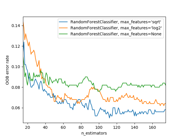
Bigger forests using a smalle subset of features tens to be better (see chart below)

How to get the predictions for a SINGLE tree?

tree_preds = np.stack(
    [t.predict(valid_xs.values) for t in m.estimators_]
)  # added .values (see: https://stackoverflow.com/a/69378867)

r_mse(tree_preds.mean(0), valid_y)

0.232215

How does n_estimators impact model performance?

To answer this, we can increment the number of trees we use in our predictions one at a time like so:

plt.plot([r_mse(tree_preds[: i + 1].mean(0), valid_y) for i in range(40)])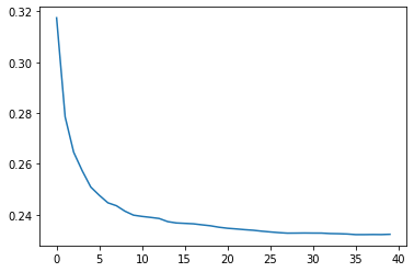

Tip

Use the above technique to determine a good range of trees to try.

Step 2: Determine why our validation set is worse than training

Tip

Use the out-of-bag (OOB) error to determine if we’re overfitting, or if the validation set covers a different time period, or if it’s a bit of both.

“The OOB error is a way of measuring prediction error in the training dataset” based on rows not used in the training of a particular tree. “This allows us to see whether the model is overfitting, without needing a separate validation set.”

“… out-of-bag error is a little like imagining that every tree therefore also has its own validation set” based on the prediction of rows not used in its training.

Important

“This is particularly beneficial in cases where we have only a small amount of training data” (we don’t necessarily have to remove items to create a validation set).

Note

If your OOB error is << than our validation set error, “something else is causing the error”

Note

“we compoare [OOB predictions] to our training labels”since this is being calculated on trees using the training set.”

r_mse(m.oob_prediction_, train_y)

0.210601

Model Interpretation

How confident are we in our predictions using a particular row of data?

Answer: “use the standard deviation of predictions across the trees, instead of just the mean. This tells us the relative confidence of predictions”

Important

“…be more cautious of using the reulsts for rows where trees give very different results (higher standard deviations)”

Tip

This information is helpful in production where “if you were using this model to decide which items to bid on at auction, a low-confidence prediction might cause you to look more carefully at an item before you made a bid.”

preds = np.stack([t.predict(valid_xs.values) for t in m.estimators_])
preds.shape  # => (# of trees, # of predictions)

(40, 7988)

preds_std = preds.std(0)  # get rid of first dimension (the trees)

# std for first 5 rows of validation set
preds_std[:5]

array([0.25911739, 0.08550421, 0.11939131, 0.29835108, 0.16490343])

Which columns are the strongest predictors (and which can we ignore)?

“It’s not normally enough to just know that a model can make accurate predictions - we also want to know how it’s making predictions”

Answer: “feature importances give us this insight.”

def rf_feature_importance(m, df):
    return pd.DataFrame(
        {"cols": df.columns, "imp": m.feature_importances_}
    ).sort_values("imp", ascending=False)


def plot_fi(fi_df):
    return fi_df.plot("cols", "imp", "barh", figsize=(12, 7), legend=False)

fi_df = rf_feature_importance(m, train_xs)

# Let's look at the 10 most important features
fi_df[:10]

	cols	imp
57	YearMade	0.186662
6	ProductSize	0.133412
30	Coupler_System	0.098091
7	fiProductClassDesc	0.071924
32	Hydraulics_Flow	0.064008
65	saleElapsed	0.050607
54	ModelID	0.049313
3	fiSecondaryDesc	0.045434
1	fiModelDesc	0.033899
31	Grouser_Tracks	0.026686

plot_fi(fi_df[:30])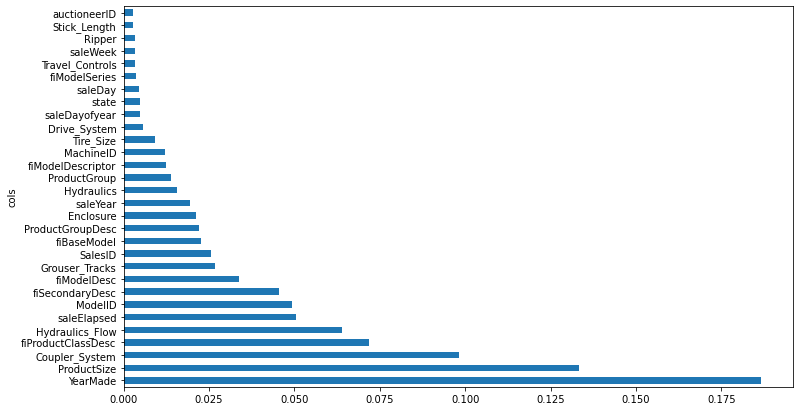

See p.304 for how feature importance is calculated.

Important

By removing variables of low importance we can still get good results while making our model simpler, more interpretable, and easier to maintain

cols_to_keep = fi_df[fi_df.imp > 0.005].cols
len(cols_to_keep)

train_xs_keep = train_xs[cols_to_keep]
valid_xs_keep = valid_xs[cols_to_keep]

m = fit_rf(train_xs_keep, train_y)

m_rmse(m, train_xs_keep, train_y), m_rmse(m, valid_xs_keep, valid_y)

(0.181366, 0.231985)

Important

Compare accuracy of full model with column subset to ensure equitable performance!

The accuracy is about the same as before, but the model is much more interpretable …

len(train_xs.columns), len(train_xs_keep.columns)

(66, 21)

plot_fi(rf_feature_importance(m, train_xs_keep[:30]))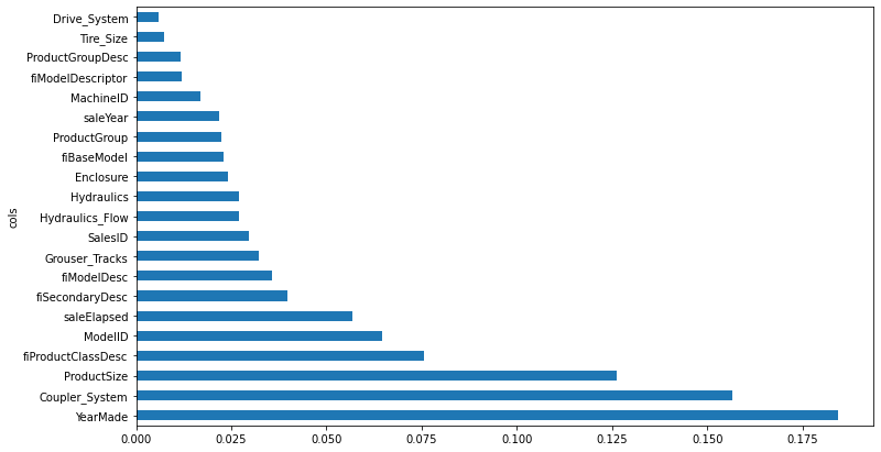

Which columns are effectively redundant?

Important

Like removing unimportant features, by removing redundant information, we make our model simpler, more interpretable, and easier to maintain

cluster_columns(train_xs_keep)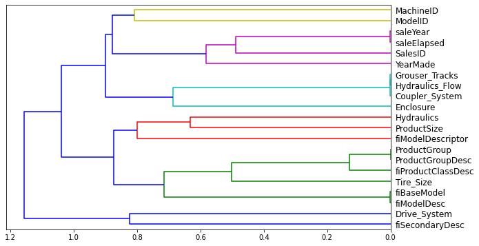

How do we determine similarity?

Important

“… the pairs of columns that are most similar are the ones that were merged together early”

“The most similar paris are found by calculating the rank correlation, which means that all the values are replaced with their rank … and then the correlation is calculated.

How do we know if a feature is “redundant” and can be dropped?

Answer: By removing potentially redundant variables one at a time

“We don’t need [the model] to be very accurate” so we can use a lower max_samples and a higher min_samples_leaf. We just want to see the effect it has by removing certain columns using the OOB score (“a number returned by sklearn that ranges between 1.0 for a perfect model and 0.0 for a random model.”

def get_oob(df, y):
    m = RandomForestRegressor(
        n_estimators=10,
        min_samples_leaf=15,
        max_samples=50_000,
        max_features=0.5,
        n_jobs=-1,
        oob_score=True,
    )
    m.fit(df, y)
    return m.oob_score_

Our baseline:

get_oob(train_xs_keep, train_y)

0.8723047876078355

Try removing redundant features one at a time:

redundant_cols = [
    "saleYear",
    "saleElapsed",
    "ProductGroupDesc",
    "ProductGroup",
    "fiModelDesc",
    "fiBaseModel",
    "Hydraulics_Flow",
    "Grouser_Tracks",
    "Coupler_System",
]

{c: get_oob(train_xs_keep.drop(c, axis=1), train_y) for c in redundant_cols}

{'Coupler_System': 0.8729675628149272,
 'Grouser_Tracks': 0.8735142839769211,
 'Hydraulics_Flow': 0.8730586366090629,
 'ProductGroup': 0.8731366740450576,
 'ProductGroupDesc': 0.8728712200071638,
 'fiBaseModel': 0.87126582392193,
 'fiModelDesc': 0.8714879359004835,
 'saleElapsed': 0.8681954238416791,
 'saleYear': 0.8713304844511609}

Now try dropping multiple variables (one from each of the tightly aligned pairs we noticed above), and compare accuracy:

cols_to_drop = ["saleYear", "ProductGroupDesc", "fiBaseModel", "Grouser_Tracks"]

get_oob(train_xs_keep.drop(cols_to_drop, axis=1), train_y)

0.8695950962336326

Assuming that its not much worse, create new DataFrames and save …

train_xs_final = train_xs_keep.drop(cols_to_drop, axis=1)
valid_xs_final = valid_xs_keep.drop(cols_to_drop, axis=1)

# save to filesystem
save_pickle(path / "train_xs_final.pkl", train_xs_final)
save_pickle(path / "valid_xs_final.pkl", valid_xs_final)

… then load them back in later

train_xs_final = load_pickle(path / "train_xs_final.pkl")
valid_xs_final = load_pickle(path / "valid_xs_final.pkl")

m = fit_rf(train_xs_final.values, train_y)
m_rmse(m, train_xs_final.values, train_y), m_rmse(m, valid_xs_final.values, valid_y)

(0.183291, 0.232867)

How do find the relationship between two predictors (columns)?

Important

Do this for the most important predictors!

First, check the count of values per category:

p = valid_xs_final["ProductSize"].value_counts().sort_index().plot.barh()
c = to.classes["ProductSize"]
plt.yticks(range(len(c)), c)

([<matplotlib.axis.YTick at 0x7f6564704d10>,
  <matplotlib.axis.YTick at 0x7f6562ce8350>,
  <matplotlib.axis.YTick at 0x7f6562b34d10>,
  <matplotlib.axis.YTick at 0x7f65645b61d0>,
  <matplotlib.axis.YTick at 0x7f656473b310>,
  <matplotlib.axis.YTick at 0x7f656473bd90>,
  <matplotlib.axis.YTick at 0x7f656473b250>],
 [Text(0, 0, '#na#'),
  Text(0, 0, 'Large'),
  Text(0, 0, 'Large / Medium'),
  Text(0, 0, 'Medium'),
  Text(0, 0, 'Small'),
  Text(0, 0, 'Mini'),
  Text(0, 0, 'Compact')])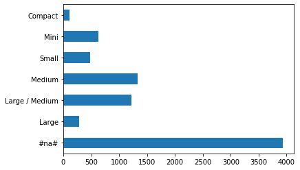

x = valid_xs_final["YearMade"].hist()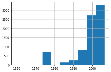

Second, built a partial dependence plot

Note

“Partial dependence plots answer the question: if a row varied on nothing other than the feature in question, how would it impact the dependent variable?

See pp.309-10 for info on how to do this, but in essence, we are attempting to isolate the effects of changes to a single variable.

from sklearn.inspection import PartialDependenceDisplay

fig, ax = plt.subplots(figsize=(12, 4))
PartialDependenceDisplay.from_estimator(
    m, valid_xs_final, ["YearMade", "ProductSize"], grid_resolution=20, ax=ax
)

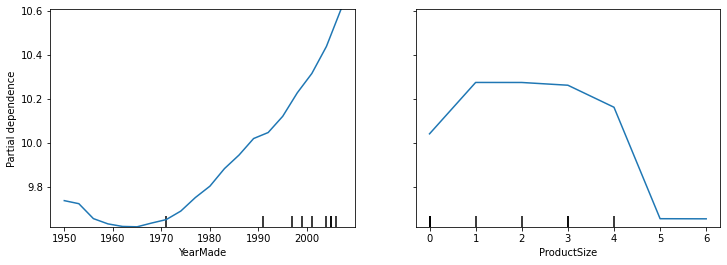
Intrepretation

The “YearMade” plot makes sense as it shows a linear relationship with price (“remember that our dependent variable is after taking the logarithm, so this means that in practice there is an exponential increase in price). Again, this is expected given that depreciation =”a multiplicative factor over time … varying year made ought to show an exponential relationship to sales price”

The “ProductSize” should raise concerns, “it shows that for the final group, which we saw is for missing values, has the lowest price.

Important

If you see an unusual relationship like this between a variable and the target, you want to understand why there are missing values and what a missing value means!

Important

Missing values can sometimes be useful predictors

Important

Missing values can sometimes indicate data leakage.

What is “data leakage”?

“The introduction of information about the target of a data mining problem, which should not be legitimately available to mine from.” The idea is that you’re cheating by introducing something by way of the independent variables that biases your predictions favorably that you won’t be able to utlize at inference time. See p.311-12 for examples.

How to determine if you have data leakage?

From p.321 … “build a model and then …

Check whether the accuracy of the model is too good to be true.
Look for important predictors that don’t make sense in pratice.
Look for partial dependence plot results that don’t make sense in practice. (see above)

Tip

“… often a good idea to build a model first and then do you data cleaning rather than vice versa … can help you identify potentially problematic data issues.

For predicting a specific row of data, what were the most important factors and how did they influence the prediction?

Answer: Use treeinterpreter. Note that:

prediction = the prediction made by RF

bias = the prediction based on taking the mean of the dependent variable (the root model for every tree)

contributions = “tells us the total change in prediction due to each of the independent variables.

“Therfore, the sum of contributions plus bias must equal the prediction for each row!

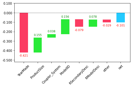
from treeinterpreter import treeinterpreter

row = valid_xs_final.iloc[:5]

pred, bias, contributions = treeinterpreter.predict(m, row.values)

pred[0], bias[0], contributions[0].sum()

(array([10.00298786]), 10.104457702350853, -0.10146984568626016)

What is the best waty to visualize this?

Answer: A waterfull plot will show us “how the positive and negative contributions from all the independent variables sum up to create the final prediction.”

import waterfall_chart

waterfall_chart.plot(
    valid_xs_final.columns,
    contributions[0],
    threshold=0.08,
    rotation_value=45,
    formatting="{:,.3f}",
)

Where is this information useful?

Answer: In production “rather than during model development. You can use it to provide useful information to users of your data product about underlying reasoning behind the predictions.”

The “Extrapolation” problem

Important

“Random forests are not able to extrapolate the types of data they have seen … that’s why we need to make sure our validation set does not contina out-of-domain data.”

See. pp.315-316.

How do determine if our “test set” is distributed in the same way as our “training set”, and if it isn’t, what columns are causing the difference?

Answer: Use a random forest where we “try to predict whether a row is in the validation set or training set.”

combined_df = pd.concat([train_xs_final, valid_xs_final])
is_valid = np.array([0] * len(train_xs_final) + [1] * len(valid_xs_final))

ood_m = fit_rf(combined_df, is_valid)

rf_feature_importance(ood_m, combined_df)[:6]

	cols	imp
5	saleElapsed	0.900343
9	SalesID	0.073015
14	MachineID	0.023312
0	YearMade	0.001036
6	ModelID	0.000405
10	Enclosure	0.000402

“This shows that three columns differ significantly between the training and validation sets: saleElapsed, SalesID, and MachineID’

See p.317 for infering what this is.

What to do with this info?

Answer: Compare the effects of removing each of these columns with the original model

m = fit_rf(train_xs_final, train_y)
print("orig:", m_rmse(m, valid_xs_final, valid_y))

orig: 0.231632

for c in ("SalesID", "saleElapsed", "MachineID"):
    m = fit_rf(train_xs_final.drop(c, axis=1), train_y)
    print(c, m_rmse(m, valid_xs_final.drop(c, axis=1), valid_y))

SalesID 0.231139
saleElapsed 0.235471
MachineID 0.229936

“… looks like we should be able to remove SaleID and MachineID without losing any accuracy”

time_vars = ["SalesID", "MachineID"]
train_xs_final_time = train_xs_final.drop(time_vars, axis=1)
valid_xs_final_time = valid_xs_final.drop(time_vars, axis=1)

m = fit_rf(train_xs_final_time, train_y)
m_rmse(m, valid_xs_final_time, valid_y)

0.228524

Note

“Removing these variables has slightly improved the model’s accuracy; but more importantly, it should make it more resilient over time, and eaiser to maintain and understand.”

Important

Build a model where the dependent variable is is_valid for ALL datasets!

“It can often uncovere subtle domain shift issues that you may otherwise miss.

Important

“One thing that might help in our case is simply to avoid using old data”

“Often, old data shows relationships that just aren’t valid anymore”

Important

This “shows you shouldn’t always use your entire dataset; sometimes a subset can be better.”

train_xs["saleYear"].hist()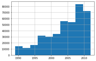

recent_sales = train_xs["saleYear"] > 2004

train_xs_recent = train_xs_final_time[recent_sales]
train_y = train_y[recent_sales]

m = fit_rf(train_xs_recent, train_y)
m_rmse(m, train_xs_recent, train_y), m_rmse(m, valid_xs_final_time, valid_y)

(0.177533, 0.229519)

Approach 3: Neural Networks

Tip

“We can leverage the work we did to trim unwanted columns in the random forest by using the same set of columns”

nn_df = pd.read_csv(path / "TrainAndValid.csv", low_memory=False)

sizes = ["Large", "Large / Medium", "Medium", "Small", "Mini", "Compact"]
nn_df.ProductSize = nn_df.ProductSize.astype("category")
nn_df.ProductSize = nn_df.ProductSize.cat.set_categories(
    sizes, ordered=True
)  # note: "inplace=True" is depreciated as of 1.30

nn_df[dep_var] = np.log(nn_df[dep_var])

nn_df = add_datepart(nn_df, "saledate")

nn_df_final = nn_df[list(train_xs_final_time.columns) + [dep_var]]

Important

Categorical columns require embeddings.

fastai uses the max_card to determine what columns should be treated as categoricals … “Embedding sizes larger that 10,000 should generaly be used only after you’ve tested whether there are better ways to group the variable”

nn_cont, nn_cat = cont_cat_split(nn_df_final, max_card=9000, dep_var=dep_var)

Important

“A categorical variable cannot, by definition, extrapolate outside the range of values that it has seen, **but we want to be able to predict auction sale prices in the future”

Therfore, “saleElapsed” needs to be made into a continous variable … which it alread is

nn_cont

['saleElapsed']

How to find the cardinality of each categorical?

nn_df_final[nn_cat].nunique()

YearMade                73
ProductSize              6
Coupler_System           2
fiProductClassDesc      74
Hydraulics_Flow          3
ModelID               5281
fiSecondaryDesc        177
fiModelDesc           5059
Enclosure                6
Hydraulics              12
ProductGroup             6
fiModelDescriptor      140
Tire_Size               17
Drive_System             4
dtype: int64

“… two variables pertaining to the ‘model’ of the equipment, both with similar very high cardinalities, suggests that they may contain similar, redundant information.”

Important

Removing rendundant columns can make your model more efficient! Try and see what the impact is.

cols_to_drop = ["fiModelDescriptor"]
train_xs_recent2 = train_xs_recent.drop(cols_to_drop, axis=1)
valid_xs_recent2 = valid_xs_final_time.drop(cols_to_drop, axis=1)

m2 = fit_rf(train_xs_recent2, train_y)
m_rmse(m2, train_xs_recent2, train_y), m_rmse(m2, valid_xs_recent2, valid_y)

(0.176776, 0.230194)

nn_cat.remove("fiModelDescriptor")

print(nn_cont)
print(nn_cat)

['saleElapsed']
['YearMade', 'ProductSize', 'Coupler_System', 'fiProductClassDesc', 'Hydraulics_Flow', 'ModelID', 'fiSecondaryDesc', 'fiModelDesc', 'Enclosure', 'Hydraulics', 'ProductGroup', 'Tire_Size', 'Drive_System']

Important

Neural networks require normalization while random forest does not because neural networks care about scaling!

nn_procs = [Categorify, FillMissing, Normalize]

nn_to = TabularPandas(
    nn_df_final, nn_procs, nn_cat, nn_cont, splits=splits, y_names=dep_var
)

Note

“Tabular models and data don’t generally require much GPU RAM, so we can use larger batch sizes”

dls = nn_to.dataloaders(bs=1024)

Tip

“it’s a good idea to set y_range for regression models

y = nn_to.train.y
y.min(), y.max()

(8.465899467468262, 11.863582611083984)

Tip

The default number of hidden layers (200,100) work well for small datasets, but should be increased if you are working with a larger dataset (500,250) for example.

from fastai.tabular.all import *

learn = tabular_learner(
    dls, y_range=(8, 12), layers=[500, 250], n_out=1, loss_func=F.mse_loss
)

learn.lr_find()

SuggestedLRs(valley=0.00015848931798245758)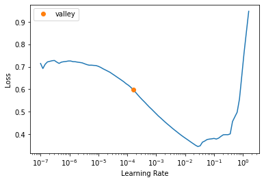

Note

There is no need to fine tune since we aren’t starting with a pretrained model.

learn.fit_one_cycle(5, 1e-2)

epoch	train_loss	valid_loss	time
0	0.062468	0.063260	00:15
1	0.053739	0.074410	00:15
2	0.047957	0.055398	00:15
3	0.042492	0.050278	00:15
4	0.039967	0.050096	00:14

preds, targs = learn.get_preds()
r_mse(preds, targs)

0.223821

learn.save("nn")

Path('models/nn.pth')

Approach 4: Boosting

Here “we add models instead of averaging them” (as compared to ensembling). See p.323-24 for all the details, but here’s how it works in general:

Train small model that underfits
Get predictions for model from #1
Get the “residuals” (‘the error for each point in the training set’) by subtracting the predictions from the targets.
Go back to step 1, “but instead of using the original targets, use the residuals as the targets for training.
Continue stesp 1-4 until you need to stop (e.g., max number of trees, you start overfitting, etc…)

Steps 3-4 are the bread and butter of things.

Important

“… each new tree will be attempting to fit the error of all of the previous trees combined. Because we are continually creating new residuals by subtracting the predictions of each new tree from the residulas from the previous tree, the residuals will get smaller and smaller.”

Some go as far as saying that such models are all you need :)

XGBoost Is All You Need

Deep Neural Networks and Tabular Data: A Surveyhttps://t.co/Z2KsHP3fvp pic.twitter.com/uh5NLS1fVP
— Bojan Tunguz (@tunguz) March 30, 2022

How do you make predictions with an ensemble of boosted trees?

Answer: By calculating the predictions from each tree and then adding them all together.

Note

“… unlike with random forests, with this approach, there is nothing to stop us from overfitting …. in a boosted ensemble, the more trees you have, the better the training error becomes, and eventually you will see overfitting on the validation set.”

Important

“Unlike random forests, gradient boosted trees are extremely sensitive to the choices of these hyperparameters.”

XGBoost and sklearn’s HistGradientBooting models are legit ML models to try …

Here are my top used ML algos for tabular data problems:

1. XGBoost
2. HistGradientBoosting
3. Logistic regression/ Ridge regression
4. LightGBM
5. MLP
6. A blend of 1. And 5.
— Bojan Tunguz (@tunguz) April 22, 2022

Other things to try

Ensembling (pp.322-23)

This is a form of “bagging” where averaging the predictions of models trained using different algorithms, each of which it is reasonable to expect would produce differnt kinds of errors, would likely product better predictions.

Combining embeddings with other models (pp.324-25)

“… shows that you can get much of the performance improvement of a neural network without having to use a neural network as inference time” by using the embeddings as inputs (which are just array lookups) to small decision tree ensemble!

In summary

Tip

Start with a random forest!

“This will give you a strong baseline … can then use that model for feature selection and partial dependence analysis to get a better understanding of your data.”

Pros/Cons of each approach:

Random forests: Pros:

Easiest to train
Resiliant to hyperparameter choices
Require little preprocessing
Fast to train
Should not overfit if you have enough trees Cons:
Can be less accurate (esp. if extrapolation is required “such as predicting future time periods.”

Gradient boosting machines (GBMs): Pros:

Often more accurate than random forests Cons:
Sensitive to hyperparmeter choices
Can overfit

Neural Networks: Pros:

Can extrapolate well
Can provide good results. Cons:
Take longest time to train
Require extra preprocessing (e.g., normalization)

Resources

https://book.fast.ai - The book’s website; it’s updated regularly with new content and recommendations from everything to GPUs to use, how to run things locally and on the cloud, etc…
“Hands-On Gradient Boosting with XGBoost and scikit-learn” - Unread personally, but on my bookshelf and recommended by those in the know.
tsai - A time series/sequences focused library built on PyTorch and fastai by Ignacio Oguiza

Tabular Modeling

Categorical Embeddings

Imports

Data preparation

Step 1: Get the data

Step 2: EDA

Step 3: Preprocessing

Handling Ordinal columns

Handling Your Dependent Variable(s)

Handling Dates

Handling Strings and Missing Data

Creating our TabularPandas

Step 1: Define our continuous and categorical columns

Step 2: Define our training and validation splits

Step 3: Build our TabularPandas object

Approach 1: Decision Trees

Step 1: Define independent/dependent variables

Step 2: Build our tree

Step 3: Build other trees

A note on categorical variables

Approach 2: Random Forests

Step 1: Define your Random Forest

Step 2: Determine why our validation set is worse than training

Model Interpretation

How confident are we in our predictions using a particular row of data?

Which columns are the strongest predictors (and which can we ignore)?

Which columns are effectively redundant?

How do find the relationship between two predictors (columns)?

For predicting a specific row of data, what were the most important factors and how did they influence the prediction?

The “Extrapolation” problem

Approach 3: Neural Networks

Approach 4: Boosting

Other things to try

In summary

Resources

Creating our `TabularPandas`

Step 3: Build our `TabularPandas` object