A Journey Through Fastbook (AJTFB) - Chapter 8: Collaborative Filtering
This chapter of "Deep Learning for Coders with fastai & PyTorch". We'll explore building these models using the traditional "dot product" approach and also using a neural network, but we'll begin by covering the idea of "latent factors," which are both important for colloborative and tabular models. Lets go!


- Collaborative Filtering
- What are "latent factors" and what is the problem they solve?
- Collaborative Filtering: From Scratch (dot product)
- Interpreting Embeddings and Biases
- Collaborative Filtering: Using fastai.collab
- Embedding Distance
- Bootstrapping
- Collaborative Filtering: From Scratch (NN)
- kwargs and @delegates
- Resources
Other posts in this series:
A Journey Through Fastbook (AJTFB) - Chapter 1
A Journey Through Fastbook (AJTFB) - Chapter 2
A Journey Through Fastbook (AJTFB) - Chapter 3
A Journey Through Fastbook (AJTFB) - Chapter 4
A Journey Through Fastbook (AJTFB) - Chapter 5
A Journey Through Fastbook (AJTFB) - Chapter 6a \
A Journey Through Fastbook (AJTFB) - Chapter 6b
A Journey Through Fastbook (AJTFB) - Chapter 7
Collaborative Filtering
What is it?
Think recommender systems which "look at which products the current user has used or liked, find other users who have used or liked similar products, and then recommend other products that those users have used or liked."
The key to making collaborative filtering and tabular models, is the idea of latent factors.
What are "latent factors" and what is the problem they solve?
Remember that models can only work with numbers, and while something like "price" can be used to accurately reflect the value of a house, how do we represent numerically concepts like the day of week, the make/model of a car, or the job function of an employee?
The answer is with latent factors.
In a nutshell, latent factors are numbers associated to a thing (e.g., day of week, model of car, job function, etc...) that are learnt during model training. At the end this process, we have numbers that provide a representation of the thing we can use and explore in a variety of ways. These factors are called "latent" because we don't know what they are beforehand.
If we had something like this ...
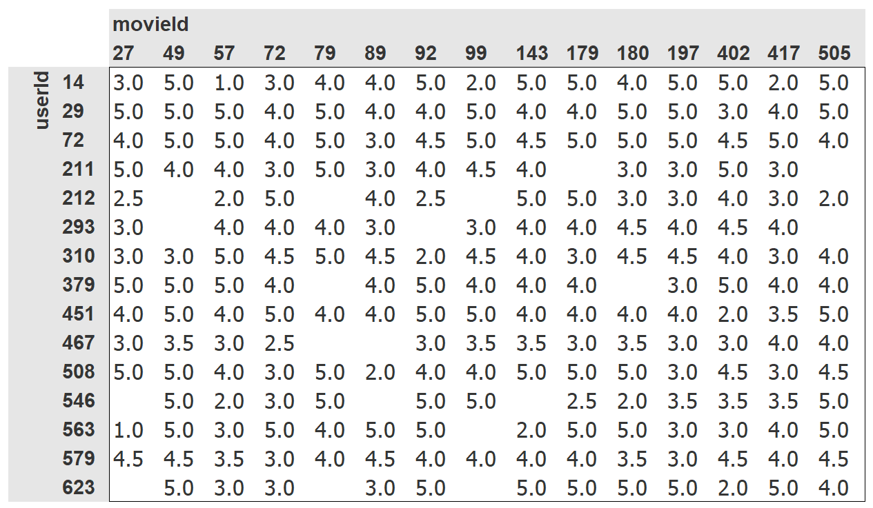
... how could we predict what users would rate movies they have yet to see? Let's take a look.
from fastai.collab import *
from fastai.tabular.all import *

path = untar_data(URLs.ML_100k)
ratings_df = pd.read_csv(path/"u.data", delimiter="\t", header=None, names=["user", "movie", "rating", "timestamp"])
ratings_df.head()
How do we numerically represent user 196 and movie 242? With latent factors we don't have to know, we can have such a representation learnt using SGD.
How do we set this up?
-
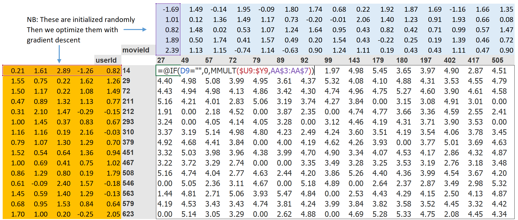
"... randomly initialized some parameters [which] will be a set of latent factors for each user and movie."
-
"... to calculate our predictions [take] the dot product of each movie with each user.
-
"... to calculate our loss ... let's pick mean squared error for now, since that is one reasonable way to represent the accuracy of a prediction"
Note: dot product = element-wise multiplication of two vectors summed up.
With this in place, "we can optimize our parameters (the latent factors) using stochastic gradient descent, such as to minimize the loss." In a picture, it looks like this ...
movies_df = pd.read_csv(path/"u.item", delimiter="|", header=None, names=["movie", "title"], usecols=(0,1), encoding="latin-1")
movies_df.head()
ratings_df = ratings_df.merge(movies_df)
ratings_df.head()
dls = CollabDataLoaders.from_df(ratings_df, item_name="title", user_name="user", rating_name="rating")
dls.show_batch()
So how do we create these latent factors for our users and movies?
"We can represent our movie and user latent factor tables as simple matrices" that we can index into. But as looking up in an index is not something our models know how to do, we need to use a special PyTorch layer that will do this for us (and more efficiently than using a one-hot-encoded, OHE, vector to do the same).
And that layer is called an embedding. It "indexes into a vector using an integer, but has its derivative calcuated in such a way that it is identical to what it would have been if it had done a matric multiplication with a one-hot-encoded vector."
n_users = len(dls.classes["user"])
n_movies = len(dls.classes["title"])
n_factors = 5

print(n_users, n_movies, n_factors)
class DotProduct(Module):
  def __init__(self, n_users, n_movies, n_factors):
      super().__init__()
      self.users_emb = Embedding(n_users, n_factors)
      self.movies_emb = Embedding(n_movies, n_factors)

  def forward(self, inp):
    users = self.users_emb(inp[:,0])
    movies = self.movies_emb(inp[:,1])
    return (users * movies).sum(dim=1)
model = DotProduct(n_users=n_users, n_movies=n_movies, n_factors=n_factors)
learn = Learner(dls, model, loss_func=MSELossFlat())

learn.fit_one_cycle(5, 5e-3)
class DotProduct(Module):
  def __init__(self, n_users, n_movies, n_factors, y_range=(0, 5.5)):
      super().__init__()
      self.users_emb = Embedding(n_users, n_factors)
      self.movies_emb = Embedding(n_movies, n_factors)
      self.y_range = y_range

  def forward(self, inp):
    users = self.users_emb(inp[:,0])
    movies = self.movies_emb(inp[:,1])
    return sigmoid_range((users * movies).sum(dim=1), *self.y_range)
model = DotProduct(n_users=n_users, n_movies=n_movies, n_factors=50)
learn = Learner(dls, model, loss_func=MSELossFlat())

learn.fit_one_cycle(5, 5e-3)
Tip 2: Add a "bias"
"One obvious missing piece is that some users are just more positive or negative in their recommendations than others, and some movies are just plain better or worse than others. But in our dot product representation, we do not have any way to encode either of these things ... **because at this point we have only weights; we don't have biases"
class DotProduct(Module):
  def __init__(self, n_users, n_movies, n_factors, y_range=(0, 5.5)):
      super().__init__()
      self.users_emb = Embedding(n_users, n_factors)
      self.users_bias = Embedding(n_users, 1)

      self.movies_emb = Embedding(n_movies, n_factors)
      self.movies_bias = Embedding(n_movies, 1)

      self.y_range = y_range

  def forward(self, inp):
    # embeddings
    users = self.users_emb(inp[:,0])
    movies = self.movies_emb(inp[:,1])

    # calc our dot product and add in biases
    # (important to include "keepdim=True" => res.shape = (64,1), else will get rid of dims equal to 1 and you just get (64))
    res = (users * movies).sum(dim=1, keepdim=True)
    res += self.users_bias(inp[:,0]) + self.movies_bias(inp[:,1])

    # return our target constrained prediction
    return sigmoid_range(res, *self.y_range)
model = DotProduct(n_users=n_users, n_movies=n_movies, n_factors=50)
learn = Learner(dls, model, loss_func=MSELossFlat())

learn.fit_one_cycle(5, 5e-3)
Tip 3: Add "weight decay"
Adding in bias has made are model more complex and therefore more prone to overfitting (which seems to be happening here).
What do you do when your model overfits?
We can solve this via data augmentation or by including one or more forms of regularization (e.g., a means to "encourage the weights to be as small as possible".
What is "weight decay" (aka "L2 regularization")?
"... consists of adding to your loss function the sum of all the weights squared."
Why do that?
"Because when we compute the gradients, it will add a contribution to them that will encourage the weights to be as small as possible."
Why would this prevent overfitting?
"The idea is that the larger the coefficients are, the sharper canyons we will have in the loss function.... Letting our model learn high parameters might cause it to fit all the data points in the training set with an overcomplex function that has very sharp changes, which will lead to overfitting.
How do we add weight decay into are training?
"... wd is a parameter that **controls that sum of squares we add to our loss" as such:
model = DotProduct(n_users=n_users, n_movies=n_movies, n_factors=50)
learn = Learner(dls, model, loss_func=MSELossFlat())

learn.fit_one_cycle(5, 5e-3, wd=0.1)
Creating our own Embedding Module
pp.265-267 show how to write your own nn.Module that does what Embedding does. Here are some of the important bits to pay attention too ...
"... optimizers require that they can get all the parameters of a module from the module's parameters method, so make sure to tell nn.Module that you want to treat a tensor as a parameters using the nn.Parameter class like so:
class T(Module):
  def __init__(self):
self.a = nn.Parameter(torch.ones(3))nn.Parameter for any trainable parameters.
class T(Module):
  def __init__(self):
    self.a = nn.Liner(1, 3, bias=False)

t = T()
t.parameters()   #=> will show all the weights of your nn.Linear
type(t.a.weight) #=> torch.nn.parameter.Parameter
Now, given a method like this ...
def create_params(size):
  return nn.Parameter(torch.zeros(*size).normal_(0, 0.01))
... we can create randomly initialized parameters, included parameters for our latent factors and biases like this:
self.users_emb = create_params([n_users, n_factors])
self.users_bias = create_params([n_users])movie_bias = learn.model.movies_bias.weight.squeeze() # => squeeze will get rid of all the single dimensions
idxs = movie_bias.argsort()[:5] # => "argsort()" returns the indices sorted by value
[dls.classes["title"][i] for i in idxs] # => look up the movie title in dls.classes
"Think about what this means .... It tells us not just whether a movie is of a kind that people tend not to enjoy watching, but that people tend to not like watching it even if it is of a kind that they would otherwise enjoy!"
To get the movies by highest bias:
idxs = movie_bias.argsort(descending=True)[:5]
[dls.classes["title"][i] for i in idxs]
See p.268 and these three StatQuest videos for more on how PCA works (btw, StatQuest is one of my top data science references so consider subscribing to his channel). Video 1, Video 2, and Video 3
learn = collab_learner(dls, n_factors=50, y_range=(0, 5.5))
learn.fit_one_cycle(5, 5e-3, wd=0.1)
learn.model
movie_bias = learn.model.i_bias.weight.squeeze()
idxs = movie_bias.argsort()[:5]
[dls.classes["title"][i] for i in idxs]
Embedding Distance
"Another thing we can do with these learned embeddings is to look at distance."
Why do this?
"If there were two movies that were nearly identical, their embedding vectors would also have to be nearly identical .... There is a more general idea here: movie similairty can be defined by the similarity of users who like those movies. And that directly means that the distance between two movies' embedding vectors can define that similarity"
movie_factors = learn.model.i_weight.weight
idx = dls.classes["title"].o2i["Silence of the Lambs, The (1991)"]
dists = nn.CosineSimilarity(dim=1)(movie_factors, movie_factors[idx][None])
targ_idx = dists.argsort(descending=True)[1]
dls.classes["title"][targ_idx]
Bootstrapping
The bootstrapping problem asks how we can make recommendations when we have a new user for which no data exists or a new product/movie for which no reviews have been made?
The recommended approach "is to use a tabular model based on user metadata to construct your initial embedding vector. When a new user signs up, think about what questions you could ask to help you understand their tastes. Then you can create a model in which the dependent variable is a user's embedding vector, and the independent variables are the results of the questions that you ask them, along with their signup metadata."
See p.271 for more information on how collaborative models may contribute to positive feedback loops and how humans can mitigate by being part of the process.
Collaborative Filtering: From Scratch (NN)
A neural network approach requires we "take the results of the embedding lookup and concatenate those activations together. This gives us a matrix we can then pass through linear layers and nonlinearities..."
How do we determine the number of latent factors a "thing" should have?
Use get_emb_sz to return "the recommended sizes for embedding matrices for your data, **based on a heuristic that fast.ai has found tends to work well in practice"
embs = get_emb_sz(dls)
embs
class CollabNN(Module):
  def __init__(self, user_sz, item_sz, y_range=(0, 0.5), n_act=100):
    self.user_factors = Embedding(*user_sz)
    self.item_factors = Embedding(*item_sz)
    self.layers = nn.Sequential(
      nn.Linear(user_sz[1] + item_sz[1], n_act),
      nn.ReLU(),
      nn.Linear(n_act, 1)
    )
    self.y_range = y_range

  def forward(self, x):
    embs = self.user_factors(x[:,0]), self.item_factors(x[:,1])
    x = self.layers(torch.cat(embs, dim=1))
    return sigmoid_range(x, *self.y_range)
model = CollabNN(*embs)
learn = Learner(dls, model, loss_func=MSELossFlat())
learn.fit_one_cycle(5, 5e-3, wd=0.1)
If we use the collab_learner, will will calculate our embedding sizes for us and also give us the option of defining how many more layers we want to tack on via the layers parameter. All we have to do is tell it to use_nn=True to use a NN rather than the default dot-product model.
learn = collab_learner(dls, use_nn=True, y_range=(0,0.5), layers=[100,50])
learn.model
learn.fit_one_cycle(5, 5e-3, wd=0.1)
Why use a neural network (NN)?
Because "we can now directly incorporate other user and movie information, date and time information, or any other information that may be relevant to the recommendation."
We'll see this when we look at TabularModel (of which EmbeddingNN is a subclass with no continuous data [n_cont=0] and an out_sz=1.
kwargs and @delegates
Some helpful notes for both are included on pp.273-274. In short ...
**kwargs:
-
**kwargsas a parameter = "put any additional keyword arguments into a dict calledkwargs" -
**kwargspassed as an argument = "insert all key/value pairs in thekwargsdict as named arguments here."
@delegates:
"... fastai resolves [the issue of using **kwargs to avoid having to write out all the arguments of the base class] by providing a special @delegates decorator, which automatically changes the signature of the class or function ... to insert all of its keyword arguments into the signature."
Resources
- https://book.fast.ai - The book's website; it's updated regularly with new content and recommendations from everything to GPUs to use, how to run things locally and on the cloud, etc...